Introduction:

Springs are crucial for maintaining rural water supply and ecosystem health in mountainous regions. In the Himalayan terrain, communities predominantly rely on perennial springs for drinking and domestic purposes. However, in recent years, numerous springs have exhibited declining discharge due to changing climate patterns, land use alterations, and increasing anthropogenic pressure. The Upper Yamuna Basin has undergone rapid land use transformation, deforestation, and urban expansion, which have adversely affected natural groundwater recharge processes. Monitoring spring discharge and associated hydro-chemical parameters is essential for understanding the current status of groundwater resources.

Objective:

This study aims to:

1. Analyze physico-chemical characteristics of spring water.

2. Assess the current spring discharge conditions (2025).

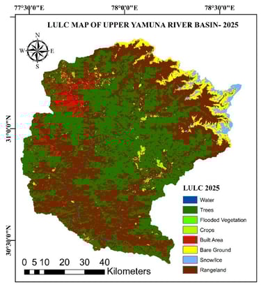
3. Examine land use/land cover changes from 2017 to 2025.

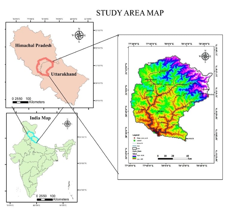
Study area:

The study area is situated within the Upper Yamuna River Basin, extending from Yamunotri in the Uttarkashi district to Dakpathar in the Dehradun district, located in the state of Uttarakhand, India.

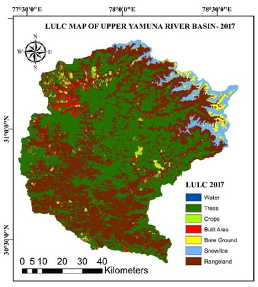
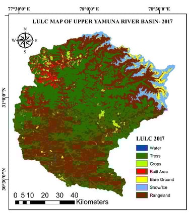
TITLE NAME: Integrated Assessment of Spring Water Quality, Land Use and Land Cover (LULC) Dynamics in the Upper Yamuna Basin, Uttarakhand

Result & Discussion

Methodology:

1. Data Collection

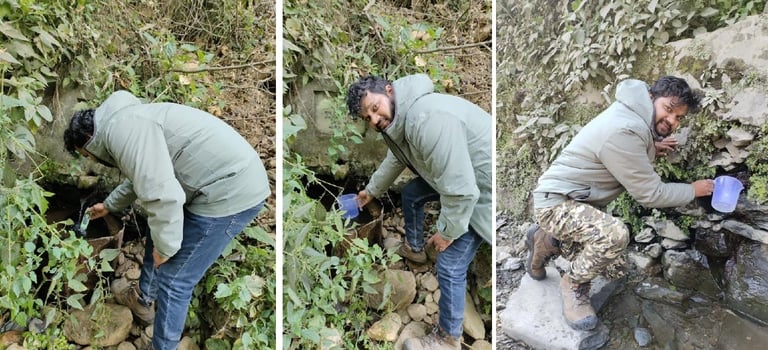
2. Field Investigation

3. In-situ water quality analysis

4. Data integration

5. Interpretation and Results

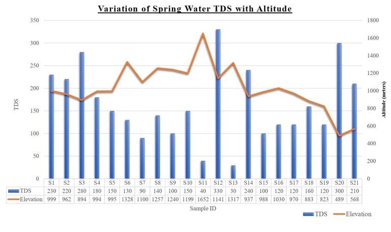
The given image represents a graphical summary of physicochemical parameters of spring water samples collected from different locations. The parameters plotted in the figure include Total Dissolved Solids (TDS), Electrical Conductivity (EC), Temperature, and Elevation (Altitude) for 21 spring samples labeled from S1 to S21.

Each sample point (S1–S21) corresponds to a specific spring location where the following parameters were measured:

• Electrical Conductivity (EC): Represented by blue bars

• Temperature: Represented by orange bars

• Total Dissolved Solids (TDS): Shown as a yellow trend line

• Elevation (Altitude): Shown as a gray trend line.

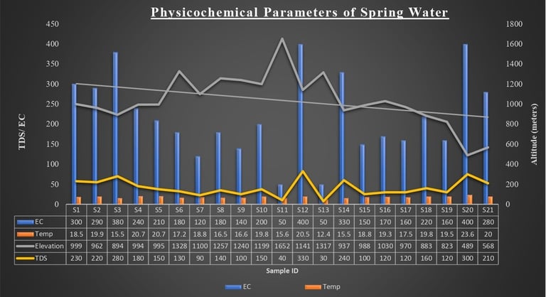
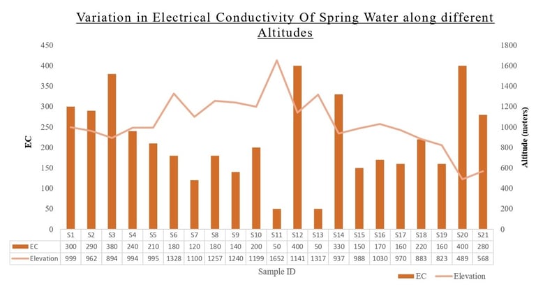
Variation of EC and TDS with Altitude

• The graph clearly shows that EC and TDS values generally decrease with increasing altitude.

• Lower altitude springs (e.g., S12, S20) tend to have higher EC and TDS values, indicating higher mineral content.

• Higher altitude springs (e.g., S7, S11) show comparatively lower EC and TDS, reflecting fresher water with less dissolved ions.

This trend suggests that water at lower elevations has had longer residence time and greater interaction with geological formations, leading to higher mineral dissolution.

• The variability among samples indicates that spring water quality is not uniform across the region.

• Differences in EC and TDS values reflect variations in:

  • Lithology

  • Recharge conditions

  • Flow paths

  • Anthropogenic influences

• The close parallel behavior of EC bars and TDS line confirms their direct proportional relationship, which is expected because TDS is largely derived from ionic content measured through EC.

1. The relationship between altitude and key water quality parameters of springs. It demonstrates that:

• TDS and EC generally decrease with increasing elevation,

• Spring water chemistry is strongly controlled by geological and topographical factors,

• Multi-parameter analysis is essential for comprehensive evaluation of groundwater resources.

Thus, Spring water quality plays a crucial role in interpreting the hydrogeochemical behavior of springs and contributes valuable insights for sustainable water resource management in mountainous terrains.

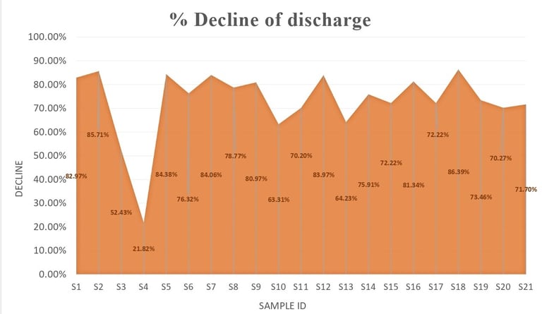
2. A substantial decline in spring discharge from 2012 to 2025, reflecting increasing stress on groundwater resources in the region. The consistent downward trend across almost all springs highlights the seriousness of the issue and emphasizes the need for:

• Immediate conservation actions

• Sustainable watershed management

• Scientific interventions to restore spring health

Thus, this figure plays a crucial role in understanding the temporal dynamics of spring systems and provides essential evidence for addressing water security challenges in the area.

3. The LULC change analysis reveals a clear shift from natural ecosystems toward human-dominated landscapes. The dominant trends include:

   • Loss of forest cover

   • Increase in built-up areas

   • Expansion of rangelands

   • Reduction in snow/ice and cropland

   These transformations indicate:

   • Growing anthropogenic pressure

   • Environmental degradation

   • Potential impacts on hydrology, biodiversity, and climate regulation

   These changes have serious environmental consequences, particularly on groundwater resources and spring sustainability. Therefore, the LULC analysis serves as a crucial tool for understanding human–environment interactions and for developing strategies toward sustainable land and water resource management.

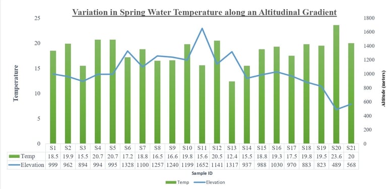
Relationship Between Temperature and Altitude

A general inverse relationship can be observed between altitude and temperature:

• Springs located at higher altitudes (e.g., S11, S7, S8) tend to show lower water temperatures.

• Springs at lower elevations (e.g., S20, S21) generally exhibit higher temperatures.

This pattern reflects the natural environmental control of altitude on groundwater temperature, which is influenced by:

• Lower ambient air temperature at higher elevations

• Reduced solar heating

• Shorter subsurface flow paths

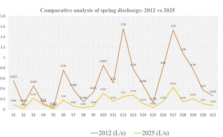
The image presents a comparative analysis of spring discharge between the years 2012 and 2025 for 21 monitored springs (S1 to S21).

The graph uses two trend lines:

• Orange line: Spring discharge in 2012 (L/s)

• Yellow line: Spring discharge in 2025 (L/s)

This visual comparison clearly illustrates the temporal change in discharge over a period of more than a decade.

• In 2012, many springs exhibited moderate to high discharge values (e.g., S12, S17, S18).

• By 2025, these values have drastically reduced, in several cases to less than half of their earlier flow.

This shows that:

• Some springs have undergone severe depletion

• Others show moderate but noticeable decline

• No spring shows improvement or increase in discharge

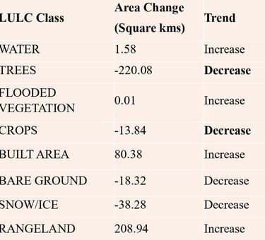
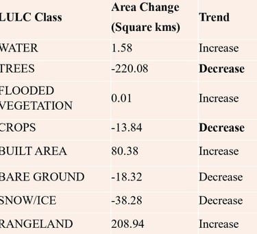
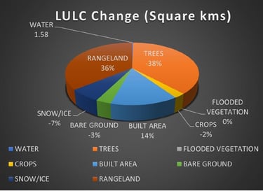
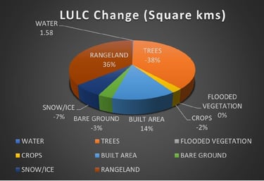
The provided images present a Land Use/Land Cover (LULC) change analysis in the form of a pie chart and an accompanying data table. Together, they illustrate how different land cover classes have changed over a specific time period in terms of area (square kilometers) and trend (increase or decrease).

A. Major Decrease in Forest Cover (Trees)

• The largest negative change is observed in the Trees category (-220.08 sq. km, -38%).

• This indicates substantial deforestation or loss of natural forest cover.

This trend suggests:

• Degradation of natural ecosystems

• Possible conversion of forest land to other uses

• Increased human pressure on natural resources

B. Significant Increase in Built-Up Area

• Built Area shows a major increase of +80.38 sq. km (14%)

This clearly reflects:

• Rapid urbanization

• Expansion of infrastructure

• Growth of settlements and construction activities

This change indicates increasing anthropogenic influence on the landscape.

C. Expansion of Rangeland

• Rangeland has increased by +208.94 sq. km (36%)

This suggests that:

• Large areas of former forests or croplands may have been converted into open grazing or degraded lands

• Land degradation and reduction in productive vegetation cover is occurring.

D. Decline in Agricultural and Natural Surfaces

• Crops decreased by -13.84 sq. km (-2%)

• Bare Ground decreased by -18.32 sq. km (-3%)

• Snow/Ice reduced by -38.28 sq. km (-7%)

The reduction in snow/ice cover may indicate:

• Effects of climate change

• Rising temperatures and glacial retreat

E. Minor Changes in Water and Flooded Vegetation

• Water area increased slightly (+1.58 sq. km)

• Flooded vegetation shows negligible increase (+0.01 sq. km)

These small changes suggest relatively stable surface water conditions compared to other classes.

Conclusion

References: 

• Beg, Z., Joshi, S. K., Singh, D., Kumar, S., & Gaurav, K. (2022). Surface water and groundwater interaction in the Kosi River alluvial fan of the Himalayan Foreland. Environmental Monitoring and Assessment, 194, 556.

• Maurya, A. K., Swarnkar, S., & Prakash, S. (2024). Hydrological impacts of altered monsoon rain spells in the Indian Ganga basin: A century-long perspective. Environmental Research: Climate, 3(1), 015010.

• Jasechko, S. (2019). Global isotope hydrogeology—Review. Reviews of Geophysics, 57. https://doi.org/10.1029/2018RG000627

• Matheswaran, K., Khadka, A., Dhaubanjar, S., Bharati, L., Kumar, S., & Shrestha, S. (2019). Delineation of spring recharge zones using environmental isotopes to support climate-resilient interventions in two mountainous catchments in Far-Western Nepal. Hydrogeology Journal, 27(6), 2181–2197.

• Ouedraogo, I., Vanclooster, M., Huneau, F., Vystavna, Y., Kebede, S., & Koussoubé, Y. (2025). Surface water–groundwater interactions in a Sahelian catchment: Exploring hydrochemistry and isotopes and implications for water quality management. Water, 17(18), 2756.

• Sheikh, H. A., Bhat, M. S., Jeelani, G., Alam, A., Ahsan, S., & Shah, B. (2025). Identification of potential spring recharge areas in the Himalayan catchment using the AHP model and stable water isotopes. Journal of Earth System Science, 134(2), 83.

• Chinnasamy, P., & Prathapar, S. A. (2016). Methods to investigate the hydrology of the Himalayan springs: A review